1.2 OBJECTIVES AND SIGNIFICANT ASPECTS
In-situ measurements over the past 35 years have yielded a wealth of
statistical information about the magnetosphere and its constituent plasma
regimes. They have also provided many examples of dynamical changes of
magnetospheric plasma parameters at specific times and places in response to
changes in the solar-wind input and to internal disturbances related to
substorms. Statistical global averages and individual events are, however, not
sufficient to understand the dynamics and interconnection of this highly
dynamic system. Fundamental questions concerning plasma entry into the
magnetosphere, global plasma circulation and energization, and the global
response of the magnetospheric system to internal and external forcing
remain unanswered. These processes occur on time scales of minutes to hours,
yet currently available statistical averages are on time scales of months to
years. Statistical studies, by their nature, never represent the magnetosphere
at any instance in time. For example, the statistical magnetopause topology derived
by Sibeck et al., [1991] was obtained from an accumulation of approximately
20 years of boundary crossings by a variety of spacecraft. However, the magnetopause
is not well represented by these average profiles. To further our understanding of
the physical processes that affect the magnetopause requires the nearly instantaneous
measurement of its topology.
To address such basic questions, IMAGE will provide global imaging of three
general magnetospheric regions: a) the magnetopause, boundary layers, cusp,
and
auroral zone; b) the plasmasphere; and c) the inner plasma sheet, ring
current,
and trapped radiation. In addition, it will provide images of near-Earth
interplanetary space. The data acquired in each of these regions will be used
to determine the global structure of the magnetosphere, characterize the
connectivity between magnetospheric regions, identify dynamic responses in
these regions, and place results in a global context with previous in-situ
measurements.
The overall objective of IMAGE is best expressed by the question: How
does
the magnetosphere respond globally to the changing conditions in the solar
wind? In fact, with all its implications, this question is a statement of
the fundamental problem facing magnetospheric physics. Unlike other
disciplines
such as astrophysics, solar physics, and to a partial extent ionospheric
physics, magnetospheric physics has not had the benefit of a global
perspective of the constituent regions under study. IMAGE will provide this
perspective for the first time. Specific questions around which the IMAGE
mission has been designed are:
1) What are the dominant mechanisms for injecting plasma into the
magnetosphere on substorm and magnetic storm time scales?
2) What is the directly driven response of the magnetosphere to solar
wind changes? and
3) How and where are magnetospheric plasmas energized, transported,
and subsequently lost during storms and substorms?
The aim of the IMAGE mission is to address these objectives in
unique ways using existing imaging techniques: neutral atom imaging (NAI)
over an energy range from 10 eV to 200 keV, far ultraviolet imaging (FUV)
at 121 - 180 nm, extreme ultraviolet imaging (EUV) at 30.4 nm, and
radio plasma imaging (RPI) over the density range from 0.1 to 105 cm-3
throughout the magnetosphere. These techniques are referred to by their initials
in the following science discussion, which is used to specify the performance requirements
of the IMAGE instruments. Figure 1.2.1 illustrates the type of magnetospheric image data
that these four techniques will acquire.
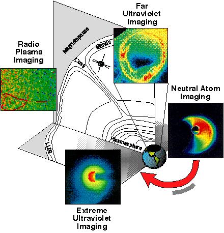
Fig. 1.2.1 Simulated IMAGE data from RPI, FUV, NAI, and
EUV.
1.2.1 Mechanisms for Injecting Plasma into the Magnetosphere
a. Solar wind plasma entry. In-situ measurements have revealed the
general structure of the magnetopause, established that it is almost
continuously in motion, and detected the existence of a boundary layer,
consisting of a mixture of magnetosheath and magnetospheric plasma with
densities intermediate between the two regions. Magnetosheath plasma has
been
shown to be accelerated as it crosses the magnetopause and to flow relatively
unimpeded through the polar cusps and down into the ionosphere [e.g.,
Smith
and Rodgers, 1991; Fuselier et al., 1991].
These observations have led to the general agreement that magnetic
reconnection
is important along the magnetopause. However, the relative global
importance of
reconnection, which produces abrupt gradients within a boundary layer of
variable thickness, and diffusive processes, which lead to generally smooth
density gradients within a boundary layer of uniform thickness, is very
uncertain. An intermediate case with a boundary layer on both closed and
open
field lines has been discussed by Lotko and Sonnerup [1994], while
Song et al. [1993] show that for northward IMF the low-latitude
boundary
layer (LLBL) shows a stair-step plasma density profile with no evidence for
plasma flow between the steps. The ability of RPI to make global
determinations
of the plasma density profiles through the boundary layer and magnetopause
is
crucially important for gaining an ultimate understanding of magnetopause
plasma entry processes.
Using HEOS-2 data, Sckopke et al. [1976] found on average a
thicker plasma mantle for northward IMF; Mitchell et al. [1987]
determined statistically that the LLBL on the flanks is thicker for southward
IMF. However, it has never been possible to compare the thicknesses of the
mantle and the LLBL simultaneously to determine if the entry of solar-wind
plasma shifts between high and low latitudes as the IMF changes. With RPI
this important simultaneous measurement will be possible, as will the
determination of whether or not the boundary layer becomes thicker around
the flanks of the magnetosphere, as claimed by Mitchell et al. [1987]
and contested by Phan and Paschmann [1995].
Recent studies indicate that the cusp at various times can be successfully
modeled either by plasma entry during quasi-steady reconnection [Onsager
et al., 1993] or by pulsed reconnection [Lockwood and Smith, 1992].
At present the relative importance of these two extremes is unclear because
temporal and spatial variations cannot be resolved by single in-situ
measurements along a spacecraft trajectory nor can they be resolved by
statistical studies. With the ability to image the density enhancement
contained within the cusp with RPI, the cusp ion population with NAI, and
the electron and proton auroras associated with the cusp with FUV, both a
steady cusp and a pulsating cusp can be resolved and characterized. In the
pulsed case a series of discrete density enhancements will be observed in
the cusp while for the quasi-steady case the enhancement will be more continuous.
b. Ionospheric ion upwelling. Another important source of plasma is
the ionosphere. The source locations of the ionospheric outflows and their
relation to the local and global ionospheric plasma and magnetic structures
and dynamics are not yet fully understood. Moore et al. [1985] have suggested
that an intense localized cusp provides the ionospheric ions for the magnetosphere,
while Shelley et al. [1985] describe the outflow region as a diffuse and extensive
region comprising the entire auroral oval. This controversy results from the dependence
up to now on statistical surveys, which use months of in-situ data and fail to resolve
spatial and temporal features on the needed time scale of minutes.
Figure 1.2.2 shows a simulated image of the charge-exchanged O+ outflow
from the cusp as will be measured by NAI. Consecutive images (with several minute
resolution) will determine the ion outflow flux and composition down to energies
of 10 eV as functions of magnetospheric activity (as defined by the FUV images of
the auroral activity and the RPI measurements of the magnetopause).
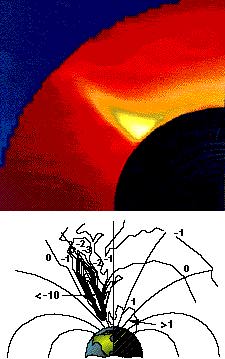
Fig. 1.2.2 (Top) simulated neutral atom image of ionospheric ion
outflow. The peak flux is approximately 105 cm-2sr-1s-1. (Bottom)
Ionospheric ion outflow model results. Contours of O+ fluxes flowing parallel
to B are shown in units of 106 cm-2s-1 down (+) and
up (-) the field line, respectively. [Horwitz, 1986].
1.2.2. Directly Driven Response of the Magnetosphere to Solar Wind
Changes
a. Magnetopause erosion and Kelvin-Helmholtz instabilities.
The most immediate effects of the solar wind on the magnetosphere arise from
its interaction with the magnetopause. Despite extensive evidence for the inward
displacement, or erosion, of the dayside magnetopause, along with a predicted
flaring of the tail magnetopause during the substorm growth phase [Coroniti
and Kennel, 1972], it has not been possible to measure the global position
of the magnetopause on the several-minute time scale needed to confirm these
effects. RPI can measure the magnetopause global position and the cusp position
while FUV monitors substorm activity, hence testing the theoretical and statistical
predictions concerning magnetopause erosion and its association with substorm activity.
Quasi-regular bright spot structures are observed in the auroral oval
afternoon sector. These auroral phenomena are part of a larger set believed to
be connected with large-scale surface waves on the LLBL [e. g., Lui et al., 1989],
which are predicted to be caused by a Kelvin-Helmholtz (K-H)
instability [e. g., Melander and Parks, 1981]. Establishing this connection
between the LLBL and the aurora and clearly identifying sources for these auroral
structures require the simultaneous measurement of auroral morphology and magnetopause
boundary layer structure and motion. RPI measurements of the boundary layer structure [Fung et al.,
1995] and irregularity scale size can be compared with periodic auroral structures
observable simultaneously by the FUV imager to determine various properties of the
predicted K-H instabilities, e. g., their spatial extent along the magnetopause.
Other phenomena, such as flux transfer events (FTEs) and pressure pulse
perturbations on the magnetopause, may have similar (but currently
undiscovered) signatures in the ionosphere. For example, Lockwood and
Smith [1992] have identified the pulsed cusp with FTEs, and the
combination of NAI imaging of the time-varying cusp ions with RPI imaging of
boundary layer structure will establish any connection between these two regions.
b. Enhanced current systems. Increased tangential stresses are
imposed
upon the magnetopause when the southward IMF component and/or the
solar wind
velocity increase. These stresses lead immediately to field-aligned currents
connecting the magnetopause to the ionosphere (the dayside region-1
currents). The currents are continued across the polar cap ionosphere and
thence by internal field-aligned currents (the region-2 currents) throughout
the magnetosphere. The internal currents are associated with plasma pressure
gradients, particularly in the plasma sheet and ring current. While the
low-altitude field-aligned currents have been computed globally from
magnetometer measurements, only very isolated measurements have been
made of the magnetospheric currents. Imaging of magnetospheric ion populations
will allow the computation of global current densities both perpendicular and
parallel to the magnetic field, i. e., the ring current and the region-2 currents,
as discussed by Roelof [1989] for isotropic pitch angle distributions.
Neutral atom images will contain information on the pitch angle distribution
of the ring current ions. This information can be used to assess the current
distribution in the magnetosphere, according to
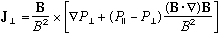
An example of this result is shown in Figure 1.2.3. For steady conditions, the
parallel current can be derived from this perpendicular current by requiring
that J = 0, and the full 3D current flow field can be inferred.
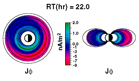
Figure 1.2.3. The azimuthal current density in the equatorial
plane and in the noon-midnight meridian Derived from a 3D ring current
simulation based on the model of Fok et al. [1995].
c. Plasmasphere erosion and refilling. The plasmapause is
traditionally considered to be the boundary between closed and open
convection trajectories. Accordingly, simple models indicate that when
the open/closed convection boundary moves inward, filled plasmasphere
flux tubes become entrained in sunward convection flow to the magnetopause
and form long tails [Rasmussen et al., 1993].
Observations suggest a more complicated picture in which outlying high-
density regions may be detached from the plasmasphere [Chappell, 1974].
Internal low-density regions may be a consequence of erosion by particle precipitation,
suggesting that as much plasma can be lost from the plasmasphere by precipitation as can
be lost by convection. Other observed dynamical features that are difficult to reconcile
with the traditional picture include nightside plasmapause steepening with increasing
Kp [Chappell et al., 1970] and rapid radial motion of density boundaries across
broad MLT sectors.
Magnetospheric imaging should be able to solve the problem of the
time-dependent structure of the plasmasphere as follows. EUV will measure
the global distribution of He+ in the inner magnetosphere in
sequences of two-dimensional, line-of-sight images. RPI will identify internal
density structures such as biteouts, closely wrapped tails, or field-aligned
density structures, which would otherwise be obscured in integrated EUV images.
Ring current images from the NAI will identify ring current-plasmasphere interactions,
and the entire set of images will be placed in context with magnetospheric activity
through FUV observations of auroral
morphology.
1.2.3 Energization and Loss of Magnetospheric Plasmas
a. Ring current injection. McIlwain [1974], using ATS-5 data,
suggested that large transient electric fields inject fresh particles into a
region outside a sharp boundary during substorms. Later Sauvaud and
Winckler [1980] showed the impulsive, dispersionless plasma injections
observed by ATS-1 and ATS-6 to be associated with the magnetic
reconfiguration
of the tail toward a more dipolar configuration. Moore et al. [1981]
then used ATS-6 and SCATHA data to measure plasma injection front
velocities in
the range of 10-100 km/s, which they attributed to the induced electric field
of the earthward propagating compression waves observed by Russell and
McPherron [1973]. Moore et al. [1981] were able to use
dual-satellite measurements to determine that the electron injection
signature
is produced mainly by a boundary motion rather than by local acceleration of
plasma. However, some evidence was found for plasma heating, which
accumulates
during a series of injection front passages. Recently Jacquey et al.
[1993] associated earthward-moving injection fronts with a disruption of the
cross-tail current at 6-9 RE, which propagates tailward with a velocity of
150-250 km/s and also propagates longitudinally during the substorm
expansion
phase.
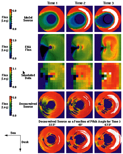
Figure 1.2.4 Simulation of a ring current injection in the
nightside
magnetosphere, in 1.7 keV ion flux (left), neutral atom flux (center), and ENA
image counts (right), for a 120 sec. exposure by NAI from the IMAGE
orbit.
The ionosphere contributes significantly to the energetic ion
population of the magnetosphere. For example, Daglis et al. [1990] demonstrated
a large enhancement of O+ ions in the near-Earth nightside magnetosphere
during the substorm growth phase. However, in order to determine the respective roles
of ionospheric ion injection, in-situ ion acceleration, and earthward ion transport
during substorm injections, it will be necessary to obtain composition-resolved images
of the ion populations in the near-Earth plasma sheet and ring current regions over an
energy range extending from very low values characteristic of the ionosphere up to energies
of tens of keV. Figure 1.2.4 shows the results of a simulated ring current injection for
a magnetic storm. The three panels show the ring current ions, the neutral atom population
resulting from charge exchange, and the image that would be obtained with the NAI
instrumentation on IMAGE.
b. Ring current dissipation. Storm energy, initially resident in the
ring current, is lost to energetic neutral atoms and to the aurora. The charge
exchange process between ring current ions and the geocorona is believed to
be the dominant loss mechanism. Pitch-angle diffusion of ring current ions,
leading to precipitation, is due to collisions with the low-energy plasma of
the plasmasphere and to wave-particle interactions. Through correlated study
of auroral images from FUV, plasmasphere images from EUV and RPI, and hot plasma
images from NAI, an assessment can be made of the importance of plasma waves in
the loss of the ring current.
1.2.4 Interstellar Neutrals and Coronal Mass Ejections (CMEs).
Although
primarily magnetospheric imaging techniques, NAI and RPI will acquire
important
data on phenomena exterior to the magnetosphere.
a) The isotopic composition of interstellar H and He. Most attempts
to determine the interstellar neutral composition use the charge-exchanged
component to deduce the interstellar density. NAI will make the first direct
measurements of the isotopic composition of interstellar H and He neutrals
at Earth. These neutrals are distinguished from ambient magnetospheric
neutrals by their arrival direction (from the solar apex direction) and low energy
(~10-200 eV). Long-term measurements will allow the first direct detection of the
deuterium abundance in the local interstellar gas, which is important for understanding
the early history and geochemical evolution of the solar system and interstellar medium.
b) Use of CME-related neutral H fluxes and type II radio bursts for early
warning of geomagnetic storms? CMEs cause geomagnetic storms as they
pass the Earth. As they propagate away from the Sun, CMEs produce high energy neutrals
[Hsieh et al., 1992a] and Type II radio bursts, some of which travel ahead of
the CMEs. NAI will detect the CME-produced neutral H flux at keV energies. Similarly,
RPI observations of Type II radio bursts will occur up to 40 hours before CME arrival.
Thus, IMAGE will offer the previously unavailable early warning of severe geomagnetic
storms that seriously upset spacecraft, power grids, and communications.
1.3 APPROACH
Our approach to the IMAGE investigation has been to evaluate the science
objectives with extensive modeling in order to establish a set of performance
parameters for the various imaging techniques (NAI, FUV, EUV, and RPI). In
some cases (FUV and NAI), more than one sensor technology is required, and the
different sensors are combined within a single instrument. An optimum polar orbit
with 500 km perigee and 7 Earth radii apogee altitudes, which is
initially at a latitude of 45 degrees north in the dusk meridian, has been
chosen. Finally, we have adopted an integrated mission philosophy (Fig.
1.3.1), which begins with an existing spacecraft (FAST), within which the entire
IMAGE payload is accommodated as a single instrument in terms of the electrical
interface. The orbital strategy is to have only two data acquisition modes (high
altitude and low altitude) so that mode commanding is done
automatically based on orbital position. During mission operations the data will
be acquired by the SMEX ground station and immediately formatted for distribution
through Internet to the entire scientific community, with no proprietary data rights.
Building upon education and public outreach programs already underway by IMAGE
investigators (Connections, P. Reiff; INSPIRE, W. Taylor), we will provide
interesting and understandable results for the purpose of improving science
literacy throughout the world.
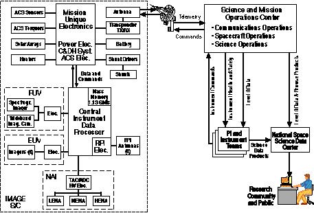
Fig. 1.3.1 IMAGE integrated mission concept uses the FAST
spacecraft architecture with existing Explorer ground systems.
A crucial part of the investigation is the proper deconvolution of the acquired
images and their adoption into well-developed magnetospheric models
through which their full impact on the discipline can be realized. In the remainder
of this section the approach to instrument selection and science closure are discussed
in order to establish clearly the investigation methodology for IMAGE.
1.3.1 IMAGE Instrument Requirements. Table 1.3.1 lists the
measurement requirements of the IMAGE Baseline Mission along with
the imagers that meet those requirements. The imagers shown between the double
horizontal lines represent the Minimum Science Mission.