2.1.1 Science Payload Summary and Measurement Requirements. To address the science questions outlined above, we have chosen a mission payload that consists of the core MI science instruments plus two additional instruments. The IMAGE instruments all communicate with the spacecraft through a centralized instrument data processor (CIDP), which causes them to appear to the spacecraft as a single instrument, greatly facilitating electrical integration.
2.1.2 Neutral Atom Imaging Instruments. A suite of three neutral atom imagers [NAI] will provide energy- and composition-resolved images at energies from 10 eV to 200 keV with a time resolution of 300 seconds. Three separate instruments are needed because the physical processes that convert neutral atoms to ions and then detect the ions differ over the three energy regimes (less than or equal to 1 keV, 1-30 keV, 10-200 keV). The optical design of each imager has been carefully tailored for individual tradeoffs of sensitivity and resolution as well as optimization of these properties across the three NAIs. All three sensors are energy/mass/angle spectrographs (i. e., they display the complete range of energy, mass, and polar angle simultaneously) rather than spectrometers (which display these parameters sequentially by scanning voltages or magnetic fields). This spectrograph approach allows instruments with modest mass and volume to achieve sensitivities attainable only with much larger and more massive spectrometers. Energy, angle, and mass resolutions are kept at the minimum needed to deconvolve anticipated particle populations whose composition (primarily H and O) and cross sections are generally well known. Angular information is obtained over 90 degree fans with less than or equal to 8 x 8 degrees resolution. Spacecraft spin is used to obtain angular information in the orthogonal (azimuthal) direction. All three instruments have narrow collimation in the azimuthal direction with collimators that consist of serrated, blackened surfaces to reduce internal scattering. The collimator deflection potentials are raised to a common value of 10 kV to deflect and absorb charged particles below 100 keV/e. Small broom magnets remove electrons with energies <200 keV. Time-of-flight (TOF) optics and electronics for all three sensors have a common heritage based on the Cassini/MIMI/CHEMS TOF and high voltage electronics.
| LENA | MENA | HENA | |
|---|---|---|---|
| Energy range [keV] | 0.01-0.3 | 1-30 | 10-200 |
| Energy resolution[[[Delta]]E/E] | 0.8 | 0.8 | 0.7 |
| FOV [deg] | 8 x 90 | 8 x 90 | 8 x 90 |
| Pixel resolution [deg] | 8 x 8 | 8 x 8 | 4 x 6 |
| Total G-factor[cm2sr] | 0.2 | 0.33 | 17.6 |
| Pixel sensitivity [cts/atom cm2sr eV/eV] | 7x10⁻⁴ | 1.6x 10⁻³ | 2x10⁻⁵ |
| Image time [s] | 300 | 300 | 300 |
| Pixel array dimensions* | 2Mx4Ex11A | 2Mx4Ex11A | 2Mx4Ex11A |
| UV rejection | 10-7 | 10-7 | 10-9 |
| Electron rejection | 10-10 | 10-9 | 10-5 |
| Ion rejection | 10-8 | 10-8 | 10-5 |
Table 2.1.1 summarizes NAI performance parameters. Pixel sensitivity relates the number of counts detected in one second to the external neutral atom flux falling on that pixel. Array dimensions refer to the number of mass (M), energy (E), and polar angle (A) channels. Common sensor design features include similar MCP detectors, anodes and image encoders; collimator and detector high voltages; and time-of-flight (TOF) electronics design.
An important part of the NAI system is the team's ability to calibrate the sensors accurately. Facilities already exist at SwRI, GSFC, LPARL, and University of Denver to achieve an accurate inter-calibration. For example, the University of Denver facility is, to our knowledge, the only facility that can provide well-known fluxes of both H and O neutrals at energies below 100 eV.
a. Low Energy Neutral Atom [LENA] imager. We have examined in detail the merits of three possible techniques for detecting neutrals in the energy range below several hundred eV: direct neutral detection without ionization [Roelof, 1987; Scime et al., 1994], ionization using an ultra-thin carbon foil [McComas et al., 1991], and ionization using surface conversion [Herrero and Smith, 1992; Gruntman, 1991; Wurz et al., 1993]. Direct detection of neutrals at low energies cannot determine the neutral atom energy and mass. At energies < 1 keV the ionization efficiency of thin foils rapidly decreases below usable levels while scattering in the foil increases. We find that the only viable technique at energies well below 1 keV is surface conversion.
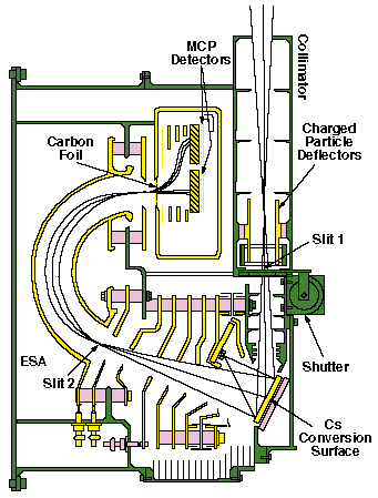
LENA combines spaceflight-proven plasma analyzer techniques with well-established, high-efficiency cesiated neutral-to-negative-ion surface conversion technology to measure composition and energy spectra of neutral atoms at 10-300 eV. LENA mass resolution [m/[[Delta]]m] of about 4 is sufficient to separate the major species of interest: H, D, 3He, 4He, and O. LENA [Ghielmetti et al., 1994] consists of a collimator, conversion unit, extraction lens, dispersive energy analyzer, and TOF mass analyzer with position-sensitive particle detection (Figure 2.1.1). LENA's high geometric factor, 0.2 cm2 sr, is achieved by simultaneously imaging in azimuthal angle, energy, and mass/charge (i. e., the spectrograph approach).
Particles enter the instrument through an aperture and traverse the baffle system described earlier. Elevation acceptance is defined by the heights of the B1 and S1 slits. A shutter located behind S1 can be closed on command to protect the conversion surface during launch and the perigee portions of the mission. LENA converts neutrals to negative ions through a near specular reflection from a low-work-function cesiated tungsten surface (at C in Fig. 2.1.1) [Wurz et al., 1995]. This technique is effective for any neutral atom with a positive electron affinity [e.g., H, O]. Conversion efficiencies as high as 67% for H [Van Wunnick et al., 1983], 66% for O [Pinxteren, 1989], and 14% for He [Veerbeck et al., 1984] have been achieved. The conversion surface is segmented to cover LENA's 90 degrees azimuthal acceptance, with the facets aligned on a conical surface centered about the instrument axis of rotational symmetry (through S1).
Fig. 2.1.1 Schematic drawing of the LENA instrument.
Laboratory testing at pressures significantly poorer than will be achieved on orbit has shown ionization efficiencies of 10-15% [Wurz et al., 1995]. Contamination of the surface will, in time, reduce conversion efficiency. Because there is a direct relationship between work function and conversion efficiency, in-situ monitoring of the work function gives conversion efficiency at any time [Wurz et al., 1995]. This is accomplished by measuring the work function using laser diodes and the photoeffect at three different wavelengths. Based on laboratory data, we conservatively estimate that surface regeneration will be required at 10-day intervals (see Fig. 2.1.2). During regeneration, the instrument shutter will be closed and the surface heated to drive out impurities. The Cs dispenser, containing a non-volatile Cs salt, is switched on to deposit the single monolayer required. To avoid contamination within the rest of the instrument, the dispenser is collimated to direct the Cs atoms to the surface. All nearby conductors are baffled.
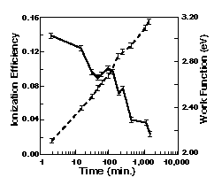
Fig. 2.1.2 Laboratory measurements of ionization efficiency (solid) and work function (dashed) for the LENA cesiated surface.
Negative ions from the Cs surface are collected by the lens, L, accelerated away from the conversion surface, and focused in the plane of the slit S2. Following the extraction lens, the negative ions are further accelerated to 20 keV between the object slit S2 and the spherical electrostatic analyzer (EA). The EA (operating at a fixed voltage) is dispersive in energy and focusing in elevation angle, so that it images the entire object slit S2 onto the foil of the TOF system.
The mass analyzer is similar to that of TIDE on Polar [Moore et al., 1995]. Secondary electrons produced on the back side of the foils are accelerated and focused onto MCP1, producing both the "start" pulse for the TOF and providing radial (energy) and polar angle information. The signal produced at MCP2 provides the "stop" pulse. The start and stop signals are obtained from 50%-transmission grids placed behind the respective MCPs. The position and TOF electronics are contained within a high-voltage bubble. The encoded information is transmitted across the HV interface via fiber optics.
The three main sources of background are UV photons, photoelectrons from the converter surface, and negative ions produced by attachment of photoelectrons to residual gas molecules. UV photons scattered at near specular angles from the conversion surface enter a light trap, while the EA provides further multiple bounce rejection. Photoelectrons from the conversion surface are separated from the negative ions and diverted into a trap by a weak magnetic field between the pole faces M1 and M2, which also traps electrons scattered through the collimator. Ion background from residual gas is minimized by accelerating photoelectrons away from the sensitive region. Any negative ions that are produced will be discriminated against by their lower energies relative to those produced on the surface.
The LENA collimator, ion optics, high voltage supplies, and TOF system are all directly derived from proven spaceflight plasma instrumentation (e. g., the Polar TIMAS [Shelley et al., 1995] and TIDE [Moore et al., 1995] instruments, and the CHEMS/MIMI/Cassini instrument. The only portion of LENA without flight heritage is the conversion surface, with which we have extensive laboratory experience [Wurz et al., 1995].
b. Medium Energy Neutral Atom [MENA] imager. The MENA imager design relies on thin carbon foils to convert neutral atoms into ions [McComas et al., 1994]. However, while McComas et al. describe an energy spectrometer (which allows only one energy to be detected at a time) MENA is an energy-mass spectrograph that samples and resolves simultaneously all energies, all angles within a 90 degree fan, and all masses. This spectrographic feature is very important for magnetospheric imaging because the weak fluxes of neutral atoms that have to be detected require an instrument with a high duty cycle. It also leads to a simpler instrument, in that the analyzer deflection potential will be fixed rather than stepped. Finally, the design is more flexible, because sensitivity can be traded off continuously with energy resolution by combining pixels in the imaging detector.
Fig. 2.1.3(A) shows an elevation view of MENA; the inset (B) shows a simplified plan view in thich the conical collimator can be seen on the left. Note that the UV filters and carbon foils are mounted on facets of a 45 degree half-angle cone. There are 5 i-,n MCPs and 5 stop MCPs with 4x3 or 4x2 pixels (depending on MCP location) corresponding to energy, polar angle position. The analyzer is a cylindrically symmetric (with axis of symmetry lying in the page) electrostatic mirror spectrograph with well-known properties [Sar-El, 1967]. The collimator consists of several parallel conical surfaces carrying alternating +10 kV and -10 kV potentials that deflect ions and electrons below 100 keV. The plates are serrated and covered with copper oxide black to reduce internal scattering. A small bar magnet just behind the collimator deflects electrons 200 keV. The other significant background that must be eliminated is ultraviolet light from the Sun and from the geocorona. Two crossed UV polarizing gratings are used to reduce UV by 10-4 while the carbon foil efficiency for secondary electrons from UV is 10-3 [Scime et al., 1994], giving a total minimum rejection of 10-7.
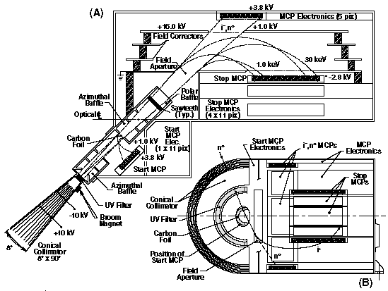
Fig. 2.1.3 MENA elevation (A) and plan (B) view schematics.
Ray paths are shown in Figure 2.1.3 for neutral atoms with energies of 1 and 30 keV, which are converted to positive ions in the carbon foil. Energy-per-unit-charge and simultaneous velocity analysis (through TOF measurement between the "start" and "stop" MCPs) yield mass per unit charge with a resolution sufficient to separate H and O. In Figure 2.1.3, secondary electrons are shown emerging from the front face of the carbon foil and electrostatically deflected onto the start MCP, which records a start pulse for TOF analysis and position for angular identification. The stop pulse is produced by the stop MCP, which also provides timing and energy (via ion arrival position on the MCP) information. In Figure 2.1.3, the cylindrical deflection volume for positive ions is located above a high-transmission (85%) grounded grid. Neutral atoms, which are not deflected by the electric field, pass through a second grid and are detected with the MCP shown near the top of the figure. Negative ions, which also emerge from the carbon foil in some fraction depending on atomic species and energy, will be accelerated by the positive deflection voltage and be deflected slightly to the left of the straight-line neutral atom trajectories and detected by the top MCP. Thus, even though the analyzer is designed for the energy and mass analysis of the atoms that emerge from the foil as positive ions, those that emerge as neutrals or negative ions can also be detected and analyzed to obtain nearly 100% of the total incident neutral fluxes (the exact fraction is obtained from calibration). This feature gives MENA a key advantage over other designs that analyze only positive or negative ions [e.g., McComas et al., 1994].
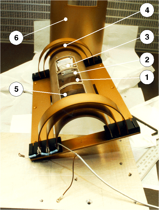
A laboratory prototype of MENA has been built and tested at SwRI with internal funds. Figure 2.1.4 shows the position of a 2.0 keV beam as a function of deflection voltage, which is equivalent to holding deflection constant and varying beam energy. Fig. 2.1.5 shows a photograph of the MENA prototype.
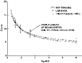
Fig. 2.1.4 Comparison of theory and laboratory data for the prototype MENA.
MENA particle optics are based on known mirror spectrograph geometries backed up by extensive ray-tracing and laboratory prototype tests. The imaging MCP and position-sensitive anode are based on TIMAS/Polar [Shelley et al., 1995], while the TOF and high voltage systems are based on Cassini/MIMI/CHEMS. This combination of a new embodiment of a well-understood and prototype-tested spectrograph with high-heritage electronics presents a minimum risk approach.
Fig. 2.1.5 Photgraph of MENA prototype. (1) mounting area for start MCP; (2) entrance region where collimator and baffle are located; (3) carbon foil covering 20 of acceptance angle; (4) field correction electrodes; (5) inner cylinder and grids at ground potentia; (6) cylindrical cover, with rectangular hole for MCP.
c. High-Energy Neutral Atom (HENA) imager. Imaging the magnetosphere in high energy (10-200 keV) neutral atoms does not require that the atoms be first ionized and then selected electrostatically (in contrast to LENA and MENA). This straight-line imaging technique does run the risk of exposing detectors to intense geocoronal EUV, while use of an EUV blocker creates the additional problem of image-blurring due to particle scattering. These are intrinsic constraints on all ENA imagers. [Hsieh et al., 1992b].
The proposed HENA imager (Fig. 2.1.6) overcomes these constraints with 1) a flight-proven TOF system for mass identification as opposed to the residual-energy method; 2) low-threshold, pixelled, solid-state detectors (SSD) that are insensitive to geocoronal EUV and are directly coupled to micro-electronics [Voss et al., 1995]); and 3) large-throughput optics with a short TOF path (2.3 cm). A total of 3440 pixels, evenly divided between two sensor heads, span a 92 degree FOV in the spacecraft meridian and 22 degrees in spacecraft azimuth (another 656 pixels are reserved for background monitoring).
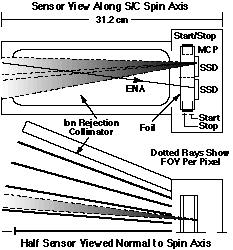
Fig. 2.1.6 HENA schematic.
The optimized EUV blocker (also to be flown on SOHO and Cassini) is a layered Si/Lexan/C foil based on Hsieh et al. [1992]. Neutrals exiting the foil cause emissions of secondary electrons that generate the start pulse for TOF. The TOF analysis acts as a coincidence system that further suppresses noise due to EUV photons. However, the foil would badly scatter particles with energies of < 200 keV. Therefore, we have chosen to use the EUV-insensitive and low-threshold pixelled SSD. The small size of each pixel (1.5 mm x 1.5 mm), its small deadlayer (range of 6 keV proton), and the short integration time of its micro-electronics (< 1 microsecond) prevent the most abundant Ly [[alpha]] photons (10.25 eV) from accumulating sufficient energy to pass the 4-keV electronic threshold (a feature made possible by the use of external J-FETs). The SSD's relative insensitivity to geocoronal emissions permits the use of a much thinner front foil (less than or equal to 5 ug/cm2 of carbon), which is still needed as a "start" electron generator. The surface of the SSD provides the electrons for the "stop" pulse. Each of the start/stop MCPs has its own foil (out of the path of the incident ENA) to further reduce the EUV scattered towards it. Because of the SSD's excellent energy resolution, the need for a long TOF path is relaxed. (A long path compounds the blurring of the image by widening the spatial spread of the incident atoms on the imaging detector).
With minimum blurring because of the removal of the EUV blocker foil and the shortened TOF path, each pixel has a well-defined FOV and geometrical factor, both set solely by the geometry of the ion-rejecting collimator and not by the statistics of particle scattering. The well-controlled partial overlapping of FOVs affords each pixel a less than or equal to 8 x 12 degrees FOV and a final angular resolution of 4 x 6 degrees. The large overall geometrical factor (1.6 cm2 sr per pixel), the high throughput (only one foil on a 90% transmission grid stands between the aperture and the SSD), and the large sensitive area of the SSD (89% as compared to 55% for an MCP) enable this instrument to achieve the desired sensitivity. Sensitivities are 0.58 for double coincidence and 0.41 for triple coincidence. As an example, we expect an average of 14-19 valid events per pixel in 5 minutes during the quiet phase of the ring current, and 100 events per pixel in 17-24 seconds during the main phase of a storm, thus providing ample statistics for proven techniques of deconvolution to reach a 4 x 6 degrees angular resolution, a quality unattainable by either SOHO or Cassini.
The HENA TOF electronics, discriminators, and fast logic are essentially copies of University of Maryland TOF electronics used on the CHEMS instrument built for Cassini/ MIMI. High voltage supplies will be copies of the CHEMSsupplies.
2.1.3 Far Ultraviolet (FUV) Imager. Science requirements that drive FUV imager designs are: 1) image the entire auroral oval from a spinning spacecraft at 7 RE apogee; 2) separate spectrally the hot proton precipitation from the statistical noise of the intense, cold geocorona.
In the FUV range, there are several bright auroral emission features that compete with the dayglow emissions. For the electron aurora, the brightest is the 130.4 nm OI auroral emission, which is multiply scattered in the atmosphere and thus cannot be used for auroral morphology studies. The next brightest is the 135.6 nm OI emission [Strickland and Anderson, 1983]. The separation of 130.4 and 135.6 nm lines necessitates the use of a spectrometer because even reflective narrow-band filter technology cannot satisfy this requirement.
The intense, cold geocorona (Lyman emissions at 121.6 nm) and the less intense, Doppler-shifted Lyman auroral emissions will be imaged separately, requiring a spectral resolution of 0.2 nm.
The IMAGE spectrographic imager achieves the high spectral resolution, high sensitivity, and high throughput required to image the electron aurora, proton aurora, and geocorona emissions. This imager is combined with a wideband imaging camera (Viking and Freja heritage) for measurement of the precipitating particle morphology with high spatial resolution and the greatest possible sensitivity, over the entire 134 - 180 nm spectral range.
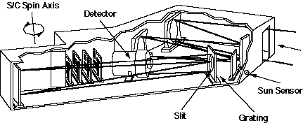
Fig. 2.1.7 Schematic of the FUV spectrographic imager.
a. Spectrographic imager. The spectrographic imager, illustrated schematically in Fig. 2.1.7, has two slits, positioned parallel to the satellite spin axis. Slit 1 is a narrow slit, 1 pixel wide, with an equivalent wavelength resolution of 0.2 nm. As shown in Fig. 2.1.8, the narrow width of this slit, combined with the 0.1 nm spectral resolution of the system, allows the imager to distinguish between, and separately measure, the central core of the Lyman [[alpha]] emissions (geocorona) and the Doppler-shifted components (proton aurora). Slit 2 is 15 pixels wide, which is equivalent to a bandwidth of 3 nm. This slit is used to separate the OI 135.6 nm emission from the brighter OI 130.4 nm emission (Fig. 2.1.8) and has a Lyman [[alpha]] blocking transmission filter. On the detector, there are two regions of interest. Region 1 contains the Lyman [[alpha]] (121.6 nm) emissions from the geocorona and proton aurora through slit 1. Region 2 contains the 135.6 nm emissions from the electron aurora through slit 2. This region actually consists of about 80% OI 135.6 nm, about 20% 135.4 nm LBH, and a negligible amount (~2%) of additional LBH at 140 nm that enters through slit 1.
The detector uses a KBr photocathode on a MgF2 window image tube with MCP intensification. The intensified image is produced on a phosphor and is fiber-optically coupled to a diode array. Diode arrays are used instead of CCDs to minimize radiation susceptibility.
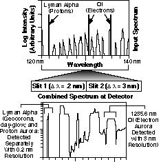
Fig. 2.1.8. Modeled UV spectrum in the 117-152 nm region and the resulting spectrum produced using the IMAGE FUV dual-slit spectrometer with two slits 5 nm apart.
The spectrographic imager is read out once per 0.1 degrees of rotation, which is equivalent to a frame rate of 30 frames/s at 0.5 rpm. There are 15 x 125 pixels on a detector region, providing a readout rate of 110 kHz. The spectrographic imager is operated in a transverse digital integration (TDI) mode: that is, the images are stored and added up in memory according to a look-up table that is dependent on the rotation rate of the spacecraft. Table 2.1.2 summarizes the characteristics of the spectrographic imager.
b. Wideband imaging camera. The wideband imaging camera uses the basic design flown on the Viking and Freja satellites (Table 2.1.2) and observes auroral LBH emissions from 134 nm to 180 nm [Anger et al., 1987]. The emission lines in this region compete favorably with the dayglow even in sunlight.
| Attribute | Spectrograph | WB Camera |
|---|---|---|
| Wavelength range | 121-140 nm | 134-180 nm |
| Focal length | 89 mm | 22.4 mm |
| Aperture dia. or area | 44 mm | 3.9 cm2 |
| FOV | 22.4 x 30deg. | |
| FOV cross track in slit | 16 deg. | |
| FOV in orbit plane | 2.5 deg. | |
| Coverage at 7 RE | 12,500 x 780 km | 27,000 x 20,000 km |
| Equivalent F/number | 2 | 1 |
| Equivalent binned pixel at 7 RE | 100 km | 50 km |
| No of pixels | 20 x 125 per [[Delta]][[lambda]]=3nm | 228 x 385 |
| Max wavelength resolution (nm) | 0.2 | N/A |
| Total counts/exp/R | 0.04 | 0.10 |
| TM rate (bits/sec) | 6000 | 4000 |
The detector in the wideband imager uses a CsI photocathode on a BaF2 window. MCPs are used to intensify the image, which is produced on a phosphor and fiberoptically coupled to a diode array (used instead of CCDs to minimize radiation susceptibility). Readout occurs once per 0.1 degrees of rotation for a frame rate of 30 frames per second at 0.5 rpm. The imaging camera data are also stored in the TDI mode. A photograph of the two wideband cameras on Freja is shown in Fig. 2.1.9.
Fig. 2.1.9 Wideband cameras on Freja.
2.1.4 He+ 30.4 nm (EUV) Imager. Effective imaging of plasmaspheric He+ requires global "snapshots" in which the high apogee of the IMAGE mission and the wide FOV of the EUV imager provide in a single exposure a map of the entire plasmasphere from the outside. Since the 1970's EUV photometers in LEO have produced "inside-out" images of the plasmasphere, showing a brightness of ~10 R. Spatial resolution of 0.2 RE and time resolution of 10 minutes are needed to resolve the structures of interest. With its sensitivity of 0.2 count/sec-pixel-R, EUV will produce high-resolution imagesof the plasmasphere.
EUV consists of three identical sensor heads (Fig. 2.1.10) serviced by a common electronics module. It employs elements of new technology, multilayer mirrors. Because it is simple and lacks moving parts, EUV is rugged and reliable. Each sensor head has a field of view of 30 x 30 degrees. The three sensors are tilted relative to one another to cover a fan-shaped field of 90 x 30 degrees. The long dimension of the field lies in the plane of the spin axis, and its center is perpendicular to the spin axis. As the satellite spins, the fan sweeps a 90 x 360 degrees swath across the sky, mapping 71% of 4[[pi]] sr.
Optics and Detector. To achieve the needed wide field and high throughput, each EUV sensor head employs a single spherical mirror. A multilayer reflective coating on the mirror selects a narrow passband around the 30.4 nm line. To circumvent the red leak in the multilayer mirror, the filter blocks H Lyman [[alpha]] contamination from the geocorona. Ray tracing shows that the spatial resolution is ~0.6 degrees, or ~0.1 RE in the equatorial plane seen from apogee. The effective spatial resolution can be adjusted to the needs of a particular experiment by summing pixels.
The detector is a dual MCP with a 2-D wedge-and-strip anode for readout. Its spherical input surface minimizes the effects of spherical aberration. For maximum quantum efficiency, an opaque alkali-halide photocathode is deposited directly onto the front surface of the MCP. The sensitivity (accounting for the duty cycle inherent in spinning) is 0.2 count/(sec pixel) per Rayleigh, where the pixel size is taken to be 0.1 RE. If we sum pixels to make a spatial resolution element (called a resel) of 0.5 RE, the count rate is 5 counts/(sec resel) per R.
Electronics. Each sensor head has its own preamplifiers and high-voltage power supply. Signals from the preamps are processed by position-finding circuitry in the central electronics module, which also includes the control microprocessor (CMP), a RAM buffer, and A/D converters for housekeeping information. The CMP accepts commands from the CIDP to select operating modes, spatial resolution, etc. The satellite provides a spin-phase sync signal to the EUV.
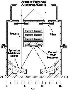
Fig. 2.1.10 Schematic of one of the three identical EUV (He+ 30.4 nm) imager sensor heads. EUV achieves high throughput and a wide field by using a large entrance aperture and a single high-efficiency reflection. Internal baffling is not shown.
Operation. A key element in the operation of the EUV is the RAM buffer, which stores a 2-D array of brightness measurements; each element in the array corresponds to a particular spatial resolution element in the sky. EUV keeps track of the satellite's spin phase, so the CMP can relate the position of each detected photon to an absolute position in the sky. It then increments the value of the corresponding array element. After a number of spins corresponding to the desired time resolution, the CIDP commands a read-out of the map buffer, compresses the image, and formats it for the telemetry stream. EUV's data rate is 1.5 kbps for about 90% of an orbit and increases to 4.5 kbps near perigee.
When the satellite is near apogee, the plasmasphere will fill about 30% of the sky. The range of the map buffer and the angular size of a resel will be set appropriately. When the satellite is near perigee, plasmaspheric emission will fill much of the sky. Then the range of the map should be increased and the angular resolution can be reduced. These and other changes in operating modes will be regulated by a mode table and selected based on orbit phase by the CIDP.
For some orientations of the spin axis, the Sun may enter the field of one of the sensor heads at some spin phases. No useful data can be recorded from the affected sensor head with the Sun in the field, and the EUV will automatically reduce the high voltage to the MCPs to avoid excessive counting rates. The filter will prevent damage to the detector by focused visible sunlight.
Heritage. The sensor heads are similar to the soft x-ray telescopes developed for the Earth-orbiting satellite Alexis. The multilayer coating techniques are now quite mature. The detector is similar to others used routinely, including examples developed by the investigators at the University of Arizona.
Calibration. The EUV will be fabricated, tested, and calibrated at the Lunar and Planetary Laboratory (LPL), University of Arizona. Calibration will utilize LPL's EUV Calibration Facility, which has been used for test and calibration of several spaceflight instruments. We will calibrate the sensor heads separately, by mounting each head in a gimbal that permits rotation about two orthogonal axes and translation along two orthogonal axes. With the entrance aperture illuminated by a collimated beam of 30.4-nm radiation of known intensity, we will record the response of the EUV as the head is rotated to probe the full field of view.
2.1.5 Radio Plasma Imager (RPI). Radio sounding has been shown to be a powerful technique for remotely observing plasma structures in the magnetosphere [Reiff et al., 1994; Green and Fung, 1994]. The feasibility of the concept was demonstrated by the success of the Alouette/ISIS topside sounders [Franklin and MacLean, 1969; Jackson et al., 1980]. The Radio Plasma Imager (RPI) is a swept frequency sounder, which transmits and receives coded electromagnetic pulses over the frequency range from 3 kHz to 3 MHz. The pulses propagate as ordinary and extraordinary mode waves through the magnetosphere and are reflected at their respective plasma cutoff frequencies. RPI measures the echo delay, Doppler spectrum, polarization, and direction as a function of sounding frequency. The Doppler spectrum allows the relative motion of the satellite and the plasma to be determined with a resolution of 400 m/s. The time resolution of the RPI is as good as 4 seconds.
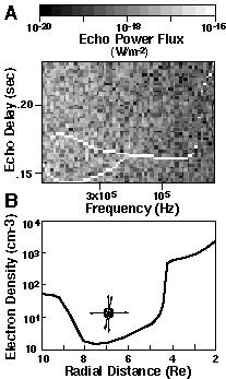
Fig. 2.1.11. A) Simulated plasmagram from RPI with 42 dB processing gain derived from B) magnetospheric density model.
The plasmagram in Figure 2.1.11 shows echo strength and delay times as functions of frequency. This simulation was based on ray tracing for the ordinary mode in a model magnetosphere. The satellite was in the noon meridian, at a latitude of 25 degrees and a geocentric distance of 7 RE. Electron density profiles can be calculated from the echo delay as a function of frequency [Huang and Reinisch, 1982]. The RPI will determine the locations and plasma densities of the magnetopause and plasmapause. The RPI will measure directions to boundary structures from a single plasmagram as well as plasma density contours from the sequence of plasmagrams along the orbit [Reiff et al., 1995]. Additional RPI information is available on the World Wide Web at the following URL address http://bolero.gsfc.nasa.gov/~green/rpi.html.
Description and Heritage. RPI is an adaptation of the state-of-the-art Digisonde Portable Sounder, (DPS) [Reinisch et al., 1992]. This well-proven design, with 18 operating worldwide, employs advanced digital techniques to investigate the bottomside ionosphere. A brassboard RPI system that was built in 1994 successfully demonstrated the feasibility to meet IMAGE requirements. The frequency range of 3 kHz to 3 MHz required for magnetospheric sounding necessitated modifications of the DPS receiver and transmitter. These frequencies measure densities from 10-1 to 105 cm-3 with a resolution of 0.1 to 10%. These densities correspond to the entire magnetosphere down to altitudes of around 1000 km, except the distant tail. The brassboard was tested at the UMass Lowell campus, with the transmitter installed at a field site 20 km away. The tests confirmed efficient transfer of RF power to the dipole antenna in the frequency range above 10 kHz. Low frequencies are mainly for local measurements, where low power is adequate.
The RPI will have two crossed 400 m tip-to-tip thin wire dipole antennas in the spin plane, ensuring adequate S/N (signal to noise) ratios. They are comparable in length to the 457 m antennas of the gravity-gradient stabilized RAE 1 and 2 spacecraft [Kaiser, 1977].
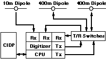
Fig. 2.1.12. RPI block diagram, showing the three receivers (Rx), two transmitters (Tx), transmit/receive (TR) switches, and the CIDP.
Two long dipoles will be driven +/-90 degrees out of phase to transmit circularly polarized waves. As sketched in Figure 2.1.12, all three orthogonal dipoles will be used for reception in order to determine the angles of arrival and polarizations of the echoes. The transmitter uses solid-state MOSFET push-pull final amplifiers with ferrite core transformers designed to cover the low frequencies. The maximum power supplied to the antennas is limited to 10 W and the maximum voltage to 3 kV. The three identical triple-conversion digitally synthesized superheterodyne receivers are space-qualified versions of the DPS design. The spatial resolution at the plasmapause and magnetopause, as observed by RPI, is shown in Figure 2.1.13. The resolution is a function of radial distance and frequency and is approximately 5 times better in the spin plane than perpendicular. The resolution of the magnetopause is also improved when compared to the plasmapause due to the focusing of the echoes. The echo arrival angles are calculated from the signal voltages on the three orthogonal antennas.
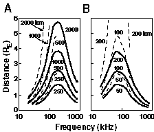
Fig. 2.1.13. The RPI spatial resolution at the magnetopause (dashed) and plasmapause (solid) in the directions A) perpendicular to the spin plane and B) in the spin plane.
Signal Processing Techniques. The large distances and the low radiated power require extensive signal processing. Two well-proven on-board digital signal processing techniques will be used to achieve the required range and angle of incidence resolution. These techniques, coherent pulse compression and Doppler integration, are routinely used for groundbased ionospheric sounding with the DPS. They provide processing gains of 9 to 42 dB. Correlating the transmitter and received pulses is called coherent pulse compression and increases the S/N ratio and decreases the effective pulse length.
Doppler integration involves repeating the pulse transmission at the same frequency and calculating separate Fourier transforms for each echo delay. This technique is routinely used to map the motions of density irregularities in the polar cap and auroral regions of the ionosphere [Reinisch et al., 1995; Reinisch, 1995]. Resolution of multiple sources will be enhanced by positive and negative Doppler shifts due to satellite motion.
Other techniques will mitigate the interference from natural magnetospheric emissions. These include frequency avoidance and agility, and polarization and spatial discrimination. Frequency agility, for example, is a technique pioneered by the DPS where the noise is measured at several closely spaced frequencies, and the frequency with the lowest noise is used for sounding. This technique will be particularly useful for avoiding discrete emissions, such as AKR.
2.1.6 Centralized Instrument Data Processor (CIDP). The CIDP consists of an array of instrument controller cards, one for each instrument, supported by a single radiation-hardened Loral Federal Systems RAD6000 SC RISC processor and a 250-Mb mass memory. The individual instrument controllers communicate with the RAD6000 processor through dual-ported memory elements connected to a command backplane. The RISC CPU acquires and processes data from the instrument controllers and transfers the processed data to the onboard mass memory system.
The CIDP, located within the RPI electronics box, communicates with the spacecraft's Mission Unique Electronics via a dedicated RS-485 serial data bus. Telemetry downlink from the CIDP is managed by a high-speed hardware controller that reads data from the mass memory, attaches the required packet headers and frame identification information, and transfers the data bit serial to the downlink transmitter. Downlink times can be preprogrammed or on ground command.
CIDP Software. VxWorks will be used as the real-time operating system for the RAD6000 processor. An IBM R-6000 work station, networked to personal computers or workstations, will serve as a centralized compiler, linker/locator as well as software configuration management tool. Excellent software development tools are available for both the UTMC 69R00 microcontrollers used on the instrument interface cards and the RAD-6000 RISC processors. Applications software for both the microcontrollers and the RAD6000 will be written in C++. IMAGE software will be developed in a controlled, structured, and well-documented manner with emphasis on software configuration control.
2.1.7 Instrument Requirements Summary. Table 2.1.3 shows the IMAGE instrument resource requirements.
| Instrument | Mass (kg) | Power (W) | Data Rate (kbps) | Dimensions (cm) | FOV(deg) | Heritage |
|---|---|---|---|---|---|---|
| NAI | ||||||
| LENA | 4.3 | 2.0 | 1.0 | 36 x 15 x 15 | 8 x 90 | TIDE (Polar) |
| MENA | 3.3 | 3.0 | 1.0 | 36 x 15 x 15 | 6 x 90 | TIDE (Polar) |
| HENA | 4.5 | 4.0 | 2.5 | 30 x 10 x 30 | 30 x 90 | CHEM (AMPTE) |
| TAC/ADC Electronics | 1.5 | 4.0 | n/a | 18 x 18 x 5 | n/a | Cassini/MIMI/CHEMS |
| HV Electronics | 2.5 | 6.0 | n/a | 18 x 18 x 8 | n/a | Cassini/MIMI/CHEMS |
| FUV | ||||||
| Spectrometer | 8.7 | 6.0 | 6.0 | 62 x 36 x 16 | 16 x 1.2 | SEPAC/AEPI |
| WB Camera | 1.9 | 3.0 | 4.0 | 26 x 15 x 13 | 22.4 x30 | Viking, Freja |
| Electronics | 2.6 | 3.0 | n/a | 15 x 20 x 16 | n/a | SOHO, TRACE |
| EUV | ||||||
| Sensors | 6.8 | 6.0 (total) | 4.5 | 15 (dia) x17 ea. | 30 x 30 | Alexis, Viking |
| Electronics | 3.5 | n/a | 15 x 15 x 10 | n/a | Alexis | |
| RPI | ||||||
| Antennas | n/a | ISEE, WIND | ||||
| X axis (2) | 3.6 ea. | 0 | 0 | 36 x 18 x 18 | ||
| Y axis (2) | 3.6 ea. | 0 | 0 | 36 x 18 x 18 | ||
| Z axis (2) | 0.55 ea. | 0 | 0 | 8.2 x 4.8 x 22.9 | ||
| Electronics,incl. CIDP | 11.0 | 11.8 | 7.0 | 36 x 27 x 14 | n/a | Digisonde Portable Sounder (DPS) |
| Totals | 66.1 | 48.8 | 26.0 |
2.2 SPACECRAFT REQUIREMENTS The IMAGE mission will use a NASA-provided spacecraft. To achieve the mission objectives, the IMAGE spacecraft must meet the following requirements:
The IMAGE spacecraft is based on the Small Explorer (SMEX) Fast Auroral Snapshot Explorer (FAST) spacecraft. FAST is an existing spacecraft of known cost which can be adapted to meet all IMAGE requirements within the MIDEX cost limit.
A design study has shown that the proposed spacecraft, based on SMEX FAST heritage designs, meets all science requirements and the MIDEX spacecraft cost limit. A sketch of the IMAGE spacecraft (as adapted from FAST) is shown in Figure 2.3.1.
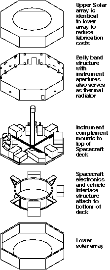
Fig. 2.3.1 Exploded view of the IMAGE spacecraft showing its FAST-based structure.
2.3.1 IMAGE Spacecraft Design Approach. FAST was chosen as a baseline spacecraft because of the similarity of the IMAGE spacecraft requirements to those of the FAST mission. Both missions require a spin-stabilized spacecraft with deployable wire booms, and both must withstand a high radiation environment. IMAGE can benefit from systems and procedures already developed for FAST. In addition, because of its simplicity, FAST has been the least expensive of all the SMEX spacecraft to date.
Because of this approach, the IMAGE spacecraft will:
All spacecraft components are copies of existing hardware (e.g., MUE) or are based on existing designs (e.g., structure). About 50% of the spacecraft subsystem costs will be for exact copies of existing hardware.
2.3.2 Spacecraft Resource Management. A significant portion of the spacecraft design effort has been directed at achieving ample margins on spacecraft resources. A minimum 20% margin has been maintained on mass, power, data rate, and inertia ratio with a 3 dB margin on downlink signal. Detailed mass and power budgets are shown in Table 2.3.1. A 20% margin has been included on total data for data storage and data transmission calculations.
| Component | Mass(kg) | Orbit Average Power (W) | Item Source or Heritage/Additional Information |
|---|---|---|---|
| Instruments | 66.1 | 48.8 | See Table 2.1.3 |
| Spacecraft Subsystems | |||
| C&DH/Electrical | |||
| Mission Unique Electronics (MUE) | 18.0 | 18.5 | FAST MUE, includes additional 3 kg shielding |
| Wire Harness & Umbilicals | 15.0 | ||
| Communications | |||
| S-band transponder | 5.1 | 5.0 | Used on ACE, TRACE, & WIRE, additional 1 kg. shielding |
| Antenna & cabling | 2.5 | Medium Gain Belt Array | |
| Power | |||
| Solar Arrays | 56.0 | 6.6 sq. m GaAs on aluminum honeycomb substrate | |
| Shunt control electronics | 1.4 | 5.0 | FAST Shunt Control Electronics |
| Battery (21A-hr) | 23.1 | MIDEX/SMEX 21 A-hr super Ni-Cad | |
| Attitude Control | |||
| ACS Torque rods | 15.4 | 5.3 | Ithaco Torqrods #D4311 (2) & #D42553 (1) |
| Magnetometer | 1.0 | SMEX 3-axis Magnetomer | |
| ACS sensors | 1.0 | FAST HCI(2) and FSS(1) | |
| Nutation damper | 5.0 | FAST-type fluid damper | |
| Mechanical | |||
| Primary structure | 33.9 | FAST-type aluminum structure | |
| Bellyband Structure | 9.0 | ||
| Radiator Battery Mount | 3.0 | ||
| Radiator Antenna Boom | 2.0 | ||
| Fasteners | 5.0 | ||
| Misc. bracketry | 5.0 | ||
| Balance weights | 5.0 | ||
| Thermal Control | |||
| Thermal blankets | 4.0 | Aluminized Kapton multi-layer insulation | |
| Heaters and thermostats | 2.0 | 10.0 | |
| Transponder heatsink | 1.1 | ||
| Spacecraft Bus Total | 213.5 | 43.8 | |
| IMAGE Total | 279.6 | 92.6 | |
| Capability | 373.0 | 129.8 | Worst case, end of life |
| Mass & power margins | 93.4 | 37.2 | ACS torquers are not used after spinup, resulting in 5.4 watts additional margin after the first 40 days of the mission. |
| Percent | 25% | 29% |
IMAGE mission operations will be carried out in the Science and Missions Operations Center (SMOC). Orbital, pointing, launch, and operational requirements for the IMAGE mission are discussed below.
2.4.1 Orbital Requirements. The required orbit for IMAGE is a 500 km x 7 RE (~ 44,600 km) altitude orbit with an inclination of 90 degrees. The initial argument of perigee is 320 degrees, placing the initial apogee at 45 degrees north latitude. Orbit analysis shows the apogee will drift over the north pole after one year and back to 45 degrees north latitude at the end of the two-year mission. The orbit right ascension of the ascending node is set at 0 or 180 degrees, placing the spacecraft spin axis at 23.5 degrees to the ecliptic plane to minimize Sun angle variation on the spacecraft. The period of the IMAGE orbit is about 13.5 hours. A Taurus Vehicle has a mass-to-orbit capability to this orbit of 373 kg.
2.4.2 Spacecraft Pointing and Attitude. The spacecraft pointing requirement is to place the spacecraft spin axis within 1 degree of the orbit plane normal, which will be performed by the spacecraft ACS prior to boom deployment. The IMAGE instruments are aligned with the centers of their fields of view perpendicular to the spacecraft spin axis. In this attitude, the instruments will scan the Earth every spacecraft revolution. Spacecraft attitude determination will be performed on board by the IMAGE ACS to within 0.1degrees for both spin angle and spin axis knowledge.
2.4.3 Communication Requirements. The IMAGE data will be transmitted as packets in a store-and-dump mode except for real-time transmissions during launch and early orbit (L&EO) and instrument checkout and calibration. The data will be stored compressed by a factor of 1.8. The telemetry rates and volumes are sized to allow automated ground operations. The telemetry protocol and formats follow the Consultative Committee for Space Data Systems (CCSDS) standards for cost-effective use of existing equipment.
The Deep Space Network (DSN) is the baseline tracking network. Scheduling of a DSN 34-m antenna will be simple because of the short downlink time relative to the length of time the spacecraft will be visible. Based on an IMAGE telemetry rate of 33.6 kb/s and a FAST spacecraft subsystems design, the DSN contact time for a data dump from the onboard solid state memory is 8 minutes per orbit (~13.5 hours) at a 2.2 Mb/s rate (including 2 kb/s of housekeeping). The solid state memory will have the ability to store one orbit's worth of data (~1.13 Gbits). All rates and times given include a 20% margin on total data. For operational simplicity, the housekeeping data will not be compressed.
2.4.4 Launch and Operational Windows. IMAGE can be launched any day of the year to attain the required orbit. The minimum launch window of one hour is only constrained by the time of day. For communications there is ample coverage for DSN northern hemisphere ground stations with contact times of about 8 hours per orbit.